
Part 2 – Benchmarking solvers
Before coding, we first introduce how to evaluate a position and how to measure and compare the performance of a Connect 4 solver.
Position’s notation
We will simply use the sequence of the played columns to code any valid Connect 4 position. The first column (left) is 1, the second column is 2, etc.
For example, the Position “4453” is:
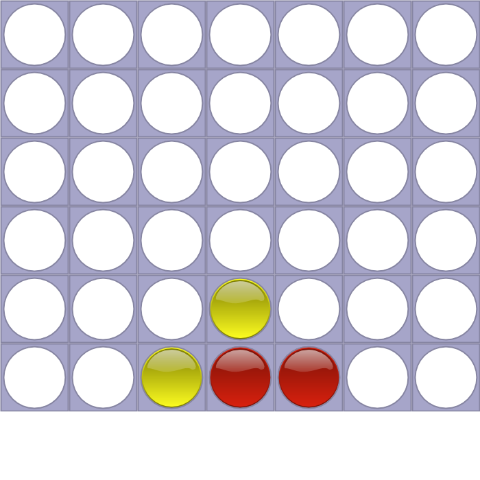
This simple notation scheme allows us to encode only valid positions that are reachable during an actual game. But bear in mind that not all sequences are valid. An invalid sequence may for example contains more than 6 times the same column, or continue after the end of the game.
Position’s score
We define a score for any non final position reflecting the outcome of the game for the player to play, considering that both players play perfectly and try to win as soon as possible or lose as late as possible. A position has:
- a positive score if the current player can win. 1 if he wins with his last stone, 2 if he wins with your second last stone and so on…
- a null score if the game will end by a draw game
- a negative score if the current player lose whatever he plays. -1 if his opponent wins with his last stone, -2 if his opponent wins with his second last stone and so on…
Positive (winning) score can be computed as 22 minus number of stone played by the winning at the end of the game. Negative (losing) score can be computed as number of stone played by the winner at the end of the game minus 22. You can notice that after playing the best move, the score of your opponent is the opposite of your score.
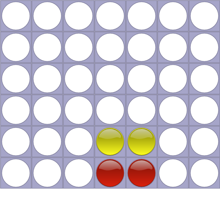
Position “4455” has a score of 18, because the current player (red) can win in two moves with his 4th stone:
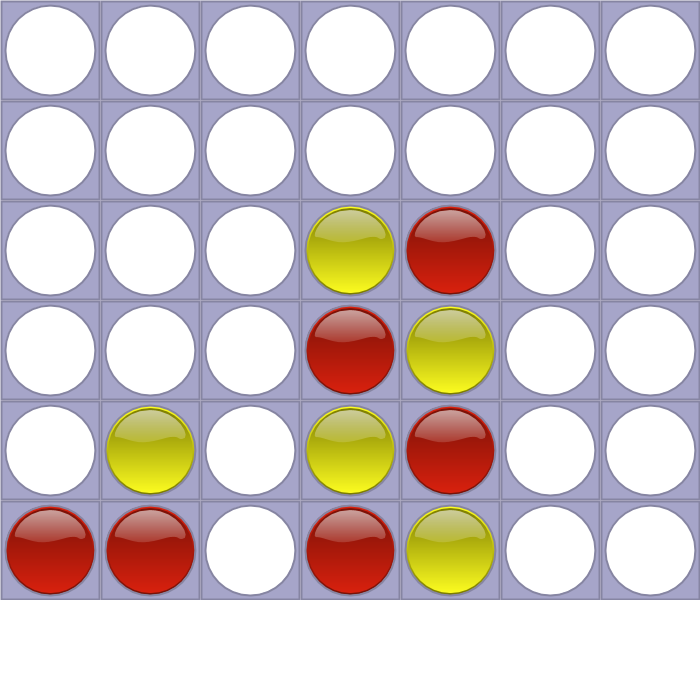
Position “44455554221” has a score of -15, because whatever current player (yellow) plays, red will win next move with his 7th stone:
Connect 4 solver benchmarking
The goal of a solver is to compute the score of any Connect 4 valid position. Weak solvers only compute the win/draw/loss outcome and strong solvers compute the score taking into account the number of moves before the end of the game.
To compare different solvers (or different versions of the same solver) we will benchmark them against the same set of positions and measure their:
- accuracy (whether the output is correct),
- execution time (on the same machine),
- number of explored positions.
Our benchmark set contains both simple and hard positions. Position are simpler to solve when we are at the end of the game, so we mixed different game depth (number of moves since the beginning of the game) and number of remaining moves before the end of the game if both players plays perfectly.
Here is our benchmark data set of 6000 positions with their expected scores:
| Test Set (1000 test cases each) | Test Set name | nb moves | nb remaining moves |
|---|---|---|---|
| Test_L3_R1 | End-Easy | 28 < moves | remaining < 14 |
| Test_L2_R1 | Middle-Easy | 14 < moves <= 28 | remaining < 14 |
| Test_L2_R2 | Middle-Medium | 14 < moves <= 28 | 14 <= remaining < 28 |
| Test_L1_R1 | Begin-Easy | moves <= 14 | remaining < 14 |
| Test_L1_R2 | Begin-Medium | moves <= 14 | 14 <= remaining < 28 |
| Test_L1_R3 | Begin-Hard | moves <= 14 | 28 <= remaining |
Each line of these test datasets contains the position and its expected score separated by a space.
First benchmark
To be able to automate our benchmarks, we requiere that the solvers follow the same simple streaming interface:
- standard input: one position per line.
- standard ouput: space separated position, score, number of explored node, computation time in microseconds.
As a first benchmark, we evaluate John Tromp’s Fhourstone solver. We used this modified version of the solver to produce the necessary output and get our first reference benchmark:
| Solver | Test Set name | mean time | mean nb pos | K pos/s |
|---|---|---|---|---|
| Fhourstone (weak solver) | End-Easy | 3.69 μs | 39.8 | 10,809 |
| Fhourstone (weak solver) | Middle-Easy | 176 μs | 2101 | 11,903 |
| Fhourstone (weak solver) | Middle-Medium | 2.41 ms | 28725 | 11,881 |
| Fhourstone (weak solver) | Begin-Easy | 209 ms | 2,456,180 | 11,752 |
| Fhourstone (weak solver) | Begin-Medium | 111 ms | 1,296,900 | 11,681 |
| Fhourstone (weak solver) | Begin-Hard | 7.95 s | 93,425,600 | 11,751 |
mean time: average computation time (per test case). mean nb pos: average number of explored nodes (per test case).